What is modern portfolio theory?
Risk is one of the most fundamental traits that is associated with every single decision we make in our day to day lives. At every turn, we are confronted with the enigmatic dance between reward and pitfall. Decisions ranging from whether you should skip dessert during dinner or not, to which borough we decide to live in are all riddled with their own potential loss and gain. The following article discusses Modern Portfolio Theory (MPT) which is one of the common ways investors use to minimise risk when investing in assets.
What is a portfolio?
https://www.investopedia.com/terms/p/portfolio.asp
A portfolio is a collection of financial investments like stocks, bonds, commodities, cash, and cash equivalents, including closed-end funds and exchange traded funds (ETFs).
MPT is a mathematical tool that explores the relationship between risk and expected return from a given portfolio. In simpler terms, it is a method for selecting investments in order to optimise for a certain outcome which can be a return or a risk target. The theory was developed and published in 1952 by Harry Markowitz and is considered as one of the most influential concepts in economics and finance.
What are the tenets of MPT?
- Rather than analysing the risk of individual assets, the framework recommends looking at the cumulative risk of a portfolio and how assets interact with each other.
- It promotes diversification as a way of minimising risk. A portfolio that is composed of a single asset or a few assets from a specific industry is likely to suffer more losses during industry-wide decline or systematic risk while a more diversified portfolio has a better chance of withstanding the contractions.
Practical starting grounds for implementing MPT

Photo by Aaron Burden on Unsplash
Let’s assume Alice recently won the lottery and wants to use MPT to build a portfolio so she can comfortably retire. One of the ways we can theoretically (as this is not an investment advice) get started with MPT is by doing an overall sector-based analysis of the stocks in the SP500. As of the writing of this article, the SP500 has 11 sectors and 503 stocks listed. We can do the sector-based analysis to determine an optimal asset allocation. Then we can dive deeper into each sector and based on deeper research, decide which stocks would be the best picks. This will help us build a diversified portfolio. However, it’s important to note that if not done carefully, this might lead to overdiversification which is one of the pitfalls of MPT.
do {sector based analysis} then {calculate asset allocation for each sector then build an optimal portfolio} |
Another approach would be to pick individual stocks and see how much of our portfolio should be allocated to each stock based on a given target return or risk amount.
List_of_stock_picks_based_on_prior_research = ["stock A", "stock B"] |
Implementation
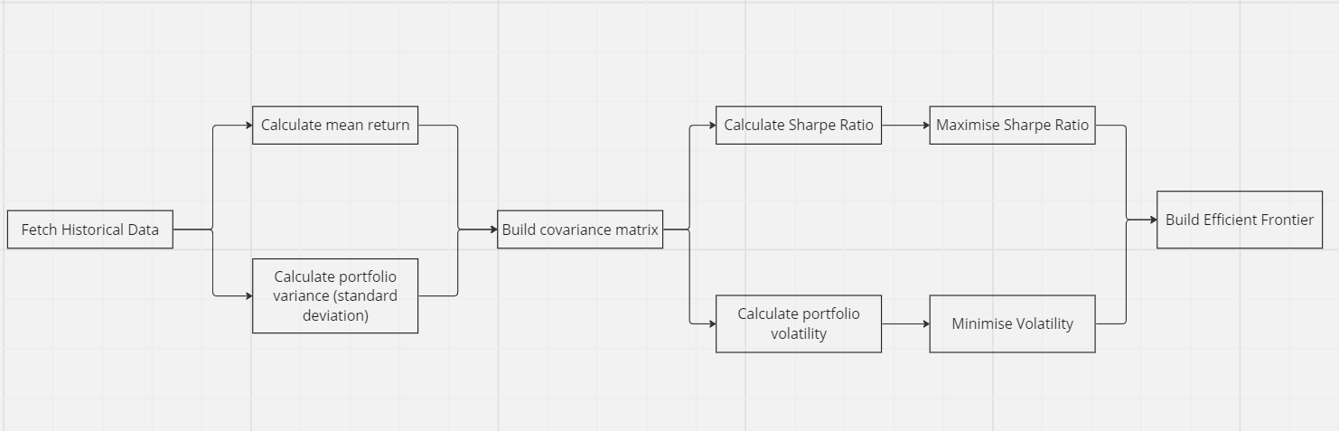
Our overall methodology for implementing MPT involves the following steps:
- Fetching historical data
- Calculating mean return
- Calculating portfolio standard deviation
- Building a covariance matrix
- Calculating Sharpe ratio
- Calculating portfolio volatility
- Maximising Sharpe ratio
- Minimising volatility
- Using max Sharpe ratio and min volatility to build Efficient frontier
Visually:
More Implementation Details
To keep the article more organised, I thought it would make sense to separate the explanation on the concepts involved in MPT from the actual code implementation. If you would like to skip straight to the code part, please go to the `Code Implementation` section. If you’re interested in the methodology and maths, stick around!
1. Fetching historical data
We can get data about the stock market using yfinance which is a free API from Yahoo.
2. Calculating mean return
We can calculate the mean return by first:
- Calculating the percentage change of the closing price for each date compared to the previous day’s closing price. Then we can calculate the mean of the percentage returns which will give us the mean return for each asset for the specified time period.
| // historical mean return for start date: 2022-08-30 and end date:2023-08-30 AAPL 0.181639 // AAPL returned 18% GOOGL 0.248391 // GOOGL returned 24% MSFT 0.251408 // MSFT returned 25% dtype: float64 |
3. Calculating portfolio standard deviation
The standard deviation of a given portfolio measures the volatility of an asset price for the given time period. A higher standard deviation implies the presence of wider price fluctuations. It takes into consideration the weight of the assets. The standard deviation of a portfolio with two assets is calculated as follows:
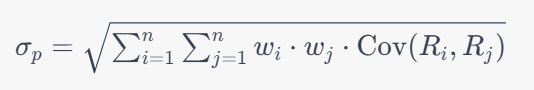
- Wi = weight of asset A,
- Wj = weight of asset B,
- Ri = Return of asset A,
- Rj = Return of asset B,
In this context, the weight of an asset refers to how much of the portfolio is made up of the asset. For example, let’s say Alice decided to invest a total of 1,000,000 USD in asset A and asset B. If she chose to invest equal amounts, she would have a portfolio that contains 500,000 USD of asset A and asset B. Wi (The weight of asset A) will be 50% and Wj (The weight of asset B) will similarly be 50%.
In the standard deviation formula, we can notice the presence of Cov(Ri, Rj) which is the covariance of the two assets. It can be calculated as follows:

Mathematical formulas can sometimes seem intimidating so let’s clarify what the above equation is. Covariance is a measure of how widely spread the values of Ri and Rj are in comparison to the mean value of Ri and mean value of Rj. Simply put, a high covariance means more noise and wide price fluctuations and vice versa.
In the above formula,
- Rit = Return of asset A for a time period t,
- Rjt = Return of asset B for a time period t,
- Ri = Average return of asset A for the time period t,
- Rj = Average return of asset B for the time period t
We have used relatively similar definitions for standard deviation and covariance in this context. The key difference is that standard deviation takes into account the weight of the assets in the portfolio. This means an asset with a higher price volatility but low weight is less likely to affect the overall gain of the portfolio.
| Date | AAPL | NVDA |
| 2023-08-28 | 180.19 | 468.35 |
| 2023-08-29 | 184.11 | 487.83 |
| 2023-08-30 | 187.64 | 492.64 |
In the above brief dataset, the mean return or percentage change would be:
MRt = (CP(t) – CP(y)) / CP(y) where,
- MRt = mean return for today’s date,
- CP(t) = today’s closing price
- CP(y) = yesterday’s closing price
The above formula can be used to calculate the mean return for each date.
| Date | AAPL | NVDA | AAPL_y | NVSA_y |
| 2023-08-28 | 180.19 | 468.35 | 0.88 | 1.77 |
| 2023-08-29 | 184.11 | 487.83 | 2.18 | 4.16 |
| 2023-08-30 | 187.64 | 492.64 | 1.91 | 0.98 |
We can take these mean values to calculate the overall mean return of the asset for the specified time period.
AAPL 9.82
NVDA 57.61
Meaning of the above numbers – AAPL and NVDA returned 9.82% and 57.61% in the given time frame.
We can then use these values as Ri and Rj in our covariance formula and Rit and Rjt as return prices for each date in our dataset.
4. Building a covariance matrix
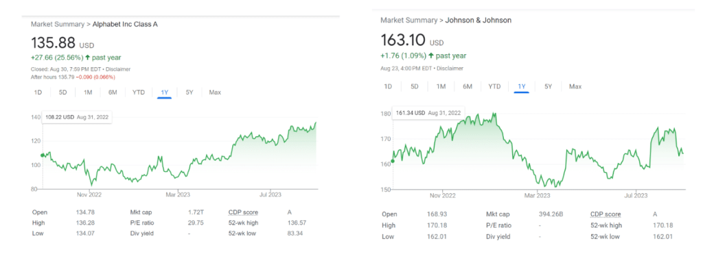
As highlighted in an earlier section, one of the most important pillars of MPT is diversification. It is a way to reduce risk in our portfolio. For example, let’s take a look at the performance of the following two stocks.
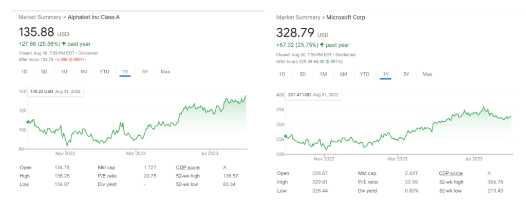
We can notice a similar price movement and uptrend.
On the contrary, let’s take a look at the charts below:
We can tell they have a relatively different price movement in comparison to the two stocks shown previously. According to MPT, having stocks with a lower correlation reduces the overall volatility of the portfolio. We can use a covariance matrix to show the relationship between price movement of any given assets. The higher the covariance, the higher the correlation.
PS – The above covariance matrix is built using the `CovarianceShrinkage(dataset).ledoit_wolf()` method from the PyportfolioOpt library.
5. Calculating Sharpe ratio
Quantifying the relationship between risk and return is the most important element in any investment. One of the most commonly used mathematical ratios to accomplish this is the Sharpe ratio.
Sharpe ratio = (Rp – Rf) / σp where,
- Rp is the average return of the portfolio,
- Rf – the risk free rate and,
- σp – the standard deviation of the portfolio.
(Rp – Rf) represents the return of the portfolio while the standard deviation signifies the volatility or risk associated with the portfolio. A higher standard deviation value means there is more variation in prices in comparison to the mean price return.
Therefore, we can see Sharpe ratio as the measure of the amount of return we get from our portfolio per unit of risk taken. A higher Sharpe ratio means the portfolio is yielding higher returns per unit of risk. Simultaneously, a negative Sharpe ratio indicates the return of the investment or portfolio is not sufficient to compensate for the level of risk it carries. There are several other mathematical ratios such as Sortino Ratio and M2 Measure which can be used to quantify the relationship between return and risk. Sharpe ratio is selected because of its wide adoption. However, it comes with its own limitations including:
- Assuming markets are normally distributed,
- Not factoring in illiquid markets which could have a relatively higher Sharpe ratio because of their low volatility,
- Nonlinear quantifiability i.e., we cannot say a portfolio with a Sharpe ratio of 4.0 yields 25% more return than a portfolio with a 3.0 ratio as the scale is not linear.
6. Calculating portfolio volatility
As alluded to in an earlier section in which we discussed standard deviation and covariance, the noise in a portfolio is the measure of its volatility.
7. Maximising Sharpe ratio / minimise negative Sharpe ratio
While talking about Sharpe ratio, we have covered what it measures and what it is used for. The pursuit of portfolio optimisation is essentially an endeavour to increase the Sharpe ratio. This means, we want to build a portfolio that has a high return for every unit of risk we take. When building a portfolio and looking into MPT and asset allocation, one half of the problem is ensuring our portfolio has the highest amount of return possible. This can be achieved mathematically by maximising our Sharpe ratio.
Portfolio optimisation is a quadratic problem which is a type of mathematical problem that involves minimising or maximising a quadratic function. The formula for portfolio optimisation is:
w=argminwσ2P=w^⊤Σw
where,
- w as the vector that minimises σ2P, and
- σ2P is equal to w⊤Σw.
σ2P is our portfolio variance(which is equal to w⊤Σw).
In w⊤Σw, w is the vector of weights and Σ is the covariance matrix of the asset returns. w⊤ means the transpose of w, which is obtained by flipping the rows and columns of w.
If we forget all the mathematical jargon, simply put, the above calculation is to essentially find how much of each asset we need to buy so we can end up with a portfolio that gives us the highest return. If Alice wants to build a portfolio that is composed of NVDA, JNJ and AAPL stocks, she can use the above formula to calculate weights that will yield the max amount of return.
Depending on the context, quadratic problems can either be convex or non-convex. If we have an objective function that is convex, the optimization problem will also become convex. The objective function is the function we use to calculate the value we are trying to optimise. In our case, the two main objective functions would be the functions we use to calculate the Sharpe ratio and portfolio variance (both functions will be included in code implementation later). Convex functions have 1 global minimum and any local minimum is equal to the global minimum. Therefore, optimisation when dealing with a convex function is about finding values that are closest or equal to the global minimum.
You may be wondering why we are talking about minimisation when we should be maximising our Sharpe ratio. Maximising Sharpe ratio is the same as minimising negative Sharpe ratio. Furthermore, the second half of our MPT problem is minimising our variance which involves applying the concepts mentioned above.
A thought worth noting in the portfolio optimisation formula (w=argminwσ2P=w^⊤Σw) is that we initially start with an arbitrary matrix of weights. The goal is to strategically traverse the convex function to arrive at a combination of weight values that bring the formula closer to its global minimum.

There are several tools we can use to minimise objective functions. Libraries such as PyTorch and Scipy provide several optimisers that can efficiently minimise objective functions. For this example, we will be using scipy’s `optimize` API.
The optimiser uses the following inputs:
| scipy.optimize.minimize(fun, x0, args=(), method=None, jac=None, hess=None, hessp=None, bounds=None, constraints=(), tol=None, callback=None, options=None) |
- fun = our objective function
- x0= initial, arbitrary weights
- args = arguments that get passed into our objective function
- method = minimisation function of our choosing
- constraints = value constraints we want to put on the optimiser
8. Minimising volatility
The first half of MPT is maximising Sharpe ratio. The second half is minimising volatility. We measure volatility using the portfolio’s standard deviation or variance. We use Scipy’s minimizer API to arrive at the minimum variance value.
9. Using max Sharpe ratio and min volatility to build Efficient frontier Portfolios
Once we have return values and weights with maximum Sharpe ratio and with minimum variance, we can create our efficient frontier.
Efficient frontier
Efficient frontier is the set of optimal portfolios that offer the highest expected return for a defined level of risk or the lowest risk for a given level of expected return.
The approach followed in this article can generate efficient frontier:
- Based on a list of assets (without a return target) and
- Based on a list of assets and given return target or a risk target
A Portfolio manager can specify the list of assets they want to invest in and a return target they expect from the portfolio. Our theoretical solution presents with an approximate asset allocation which might yield the required return.
In our example, the steps we follow to generate efficient frontier based on a list of assets involves:
- calculating the weights that give us the max Sharpe ratio
- Using these weights to calculate return1
- Calculating the weights that give us the min variance
- Using these weights to calculate return2
- Creating an array of returns based on a constant step starting from return2 to return1. E.g. return2 = 5, return1 = 15, step = 5. array_of_returns = [5, 10, 15]. Step can also be the number of portfolio allocations we want to generate. If we want to generate 10 portfolio allocations, then step would equal 10.
- For each return in array_of_returns, calculate efficient frontier given weights.
Analysis Modularity
Portfolio allocation is experimental and requires continuous iteration. The calculations we used in our analysis have other alternatives. In the table below, we can see the choice of tools we made and other alternatives we could use. Such modularity allows us to experiment with different tools and optimisers.
| Calculation/Tool | Used in | Can be replaced by/Alternatives |
| Mean return | Calculating mean return, percentage change, variance, covariance matrix | Pypfopt.expected_returns.mean_historical_return, pypfopt.expected_returns.ema_historical_return |
| pypfopt.risk_models.CovarianceShrinkage | Covariance matrix | Traditional covariance calculation |
| scipy.optimize.minimize() | Calculating max Sharpe ratio, minimising variance | Cvxpy, torch.optim |
Criticism against modern portfolio theory?
- Quant-leaning: MPT is purely quantitative and doesn’t take into account market sentiment and other qualitative factors that can influence the performance of the portfolio
- Underestimating the frequency of extreme events: It assumes market returns follow a normal distribution and doesn’t account for market downturns that can happen more often and the subsequent changes that come with them. It emphasises investing in assets that have low correlation but during these downturns, low correlations can increase significantly and portfolios can still incur heavy losses.
- The diversification curse: The pursuit of over diversification leads to incurring transaction fees. Furthermore, it might encourage adding more assets to the portfolio without a significant change in return.
- Rational investors: Similar to many economic theories, MPT assumes investors are rational and make decisions that maximise the return of their portfolios. Meanwhile, investors can choose to balance return with other factors such as influence and shared values with the cause the given company is working towards.
Final Words…
Overall, modern portfolio theory is a way of building a portfolio of assets. We can use several tools and approaches and continually iterate till we get the desired result. Furthermore, it is important to back test our models and measure the analysis accuracy to further optimise our current model. Thank you for reading this piece and ff you want to chat more, please feel free to connect with me via email at 0xnatnael@gmail.com.
Code Implementation
from typing import List, Any, Dict
import yfinance as yf
import numpy as np
import pandas as pd
from pandas import DataFrame as DataFrame
from pandas import Series as Series
from pypfopt.expected_returns import mean_historical_return, ema_historical_return
from pypfopt.risk_models import CovarianceShrinkage
from pypfopt.efficient_frontier import EfficientFrontier
import datetime as dt
from datetime import datetime as DateTime
import scipy.optimize as scOpt
from scipy.optimize import OptimizeResult
import seaborn as sns
import matplotlib.pyplot as plt


class MPT:
    def __init__(
        self,
        list_of_stocks: List[str],
        starting_date: DateTime,
        ending_date: DateTime,
    ) -> None:
        if len(list_of_stocks) == 0:
            raise ValueError("No stocks provided.")

        now_date: DateTime = dt.datetime.now()
        # check we received valid dates
        if ending_date > now_date or starting_date > now_date or starting_date >= ending_date:
            raise ValueError("Invalid date entries")

        self.list_of_stocks = list_of_stocks
        self.starting_date = starting_date
        self.ending_date = ending_date
        self.__total_number_of_assets: int | None = None
        self.__stock_close_price_data: DataFrame | None = None
        self.__covariance_matrix: DataFrame | None = None
        self.__current_sharpe_ratio: float | None = None
        self.__standard_deviation: float | None = None
        self.__TRADING_DAYS: int = 252

    def __fetch_stock_close_price_data(self) -> None:
        """
        The function fetches historical stock price data using the Yahoo Finance API and stores only the
        closing prices.
        :return: None.
        """

        # use the Yahoo Finance API to fetch historical stock price data
        data: DataFrame = yf.download(self.list_of_stocks, start=self.starting_date, end=self.ending_date)

            # we only need the closing price
        self.__stock_close_price_data = data["Close"]

    def get_stock_close_price_data(self) -> DataFrame:
        """
        The function returns the stock close price data, fetching it if necessary.
        :return: The method is returning the stock close price data, which is stored in the variable
        `self.__stock_close_price_data`.
        """
        if self.__stock_close_price_data is None:
            self.__fetch_stock_close_price_data()
        return self.__stock_close_price_data

    def __calculate_total_number_of_assets(self) -> None:
        self.__total_number_of_assets = len(self.list_of_stocks)

    def get_total_number_of_assets_in_portfolio(self) -> int:
        if self.__total_number_of_assets is None:
            self.__calculate_total_number_of_assets()
        return self.__total_number_of_assets

    def __calculate_covariance_matrix(self) -> None:
        """
        The function calculates the covariance matrix using the Ledoit-Wolf shrinkage method.
        """
        df_data_set: DataFrame = self.get_stock_close_price_data()
        self.__covariance_matrix = CovarianceShrinkage(df_data_set).ledoit_wolf()

    def get_covariance_matrix(self) -> DataFrame:
        if self.__covariance_matrix is None:
            self.__calculate_covariance_matrix()
        return self.__covariance_matrix

    def plot_correlation_heatmap(self) -> None:
        covariance_matrix: DataFrame = self.get_covariance_matrix()
        plt.figure(figsize=(10, 8))
        sns.heatmap(covariance_matrix, annot=True, cmap="coolwarm", linewidths=0.5)
        plt.title("Correlation Heatmap")
        plt.show()

    def __calculate_sharpe_ratio_given_weights(self, weights: np.ndarray) -> None:
        """
        The function calculates the Sharpe ratio given a set of weights for a portfolio.

        :param weights: The `weights` parameter represents the weights assigned to each stock in the
        portfolio. These weights determine the proportion of each stock's contribution to the overall
        portfolio return
        """
        closing_price_data: DataFrame = self.get_stock_close_price_data()
        percentage_change: DataFrame = closing_price_data.pct_change()
        simple_mean_returns: Series = percentage_change.mean() * 100
        annualised_weighted_portfolio_return: float = (
            np.sum(simple_mean_returns * weights) * self.__TRADING_DAYS
        )
        portfolio_std: float = self.get_portfolio_standard_deviation(weights=weights)
        self.__current_sharpe_ratio = (
            annualised_weighted_portfolio_return / portfolio_std
        )

    def get_sharpe_ratio_given_weights(self, weights: np.ndarray, recalculate=False) -> float:
        if self.__current_sharpe_ratio is None or recalculate:
            self.__calculate_sharpe_ratio_given_weights(weights)
        return self.__current_sharpe_ratio

    def __calculate_negative_sharpe_ratio(self, weights: np.ndarray) -> float:
        sharpe_ratio: float = self.get_sharpe_ratio_given_weights(
            weights, recalculate=True
        )
        return -1 * sharpe_ratio

    def calculate_max_sharpe_ratio(
        self,
        constraintset=(0, 1),
    ) -> OptimizeResult:
        """
        The function calculates the maximum Sharpe ratio for a given portfolio.

        :param constraintset: The `constraintset` parameter is a tuple that defines the lower and upper
        bounds for the asset weights in the portfolio. By default, it is set to `(0, 1)`, which means
        that the weights of the assets must be between 0 and 1, indicating the percentage allocation of
        :return: an OptimizeResult object.
        """
        constraints: Dict[str, Any] = {"type": "eq", "fun": lambda x: np.sum(x) - 1}
        total_num_of_assets: int = self.get_total_number_of_assets_in_portfolio()
        bounds: tuple() = tuple(constraintset for _ in range(total_num_of_assets))
        optimiser_output: Dict[str, Any] = scOpt.minimize(
            fun=self.__calculate_negative_sharpe_ratio,
            x0=total_num_of_assets * [1.0 / total_num_of_assets],
            args=(),
            method="SLSQP",
            bounds=bounds,
            constraints=constraints,
        )
        return optimiser_output

    def get_max_sharpe_ratio(self) -> float:
        return self.__calculate_max_sharpe_ratio()

    def __calculate_portfolio_standard_deviation(self, weights: np.ndarray) -> None:
        """
        The function calculates the standard deviation of a portfolio based on the given weights and
        covariance matrix.

        :param weights: The "weights" parameter represents the weights assigned to each asset in the
        portfolio. These weights determine the proportion of each asset's allocation in the portfolio
        """
        covariance_matrix: DataFrame = self.get_covariance_matrix()
        self.__standard_deviation: float = np.sqrt(
            np.dot(weights.T, np.dot(covariance_matrix, weights))
        ) * np.sqrt(self.__TRADING_DAYS)

    def get_portfolio_standard_deviation(self, weights: np.ndarray) -> float:
        if self.__standard_deviation is None:
            self.__calculate_portfolio_standard_deviation(weights)
        return self.__standard_deviation

    def __calculate_variance_for_optimisation(self, weights) -> float:
        """
        The function calculates the variance of a portfolio based on the given weights and covariance
        matrix.

        :param weights: The "weights" parameter represents a vector of weights that are used to
        calculate the variance. These weights are typically used in portfolio optimization to determine
        the allocation of assets in a portfolio. Each weight represents the proportion of the total
        investment allocated to a specific asset
        :return: the variance, which is a float value.
        """
        covariance_matrix: DataFrame = self.get_covariance_matrix()
        standard_deviation: float = np.sqrt(
            np.dot(weights.T, np.dot(covariance_matrix, weights))
        ) * np.sqrt(self.__TRADING_DAYS)
        variance: float = standard_deviation**2
        return variance

    def calculate_minimum_variance(
        self,
        constraintset=(0, 1),
    ) -> OptimizeResult:
        """
        The function calculates the minimum variance of a portfolio given a set of constraints.

        :param constraintset: The `constraintset` parameter is a tuple that defines the lower and upper
        bounds for the optimization constraints. In this case, the default value is `(0, 1)`, which means
        that the optimization constraints require the portfolio weights to be between 0 and 1 (inclusive)
        :return: The function `calculate_minimum_variance` returns an OptimizeResult object.
        """
        constraints = {"type": "eq", "fun": lambda x: np.sum(x) - 1}
        total_num_of_assets: int = self.get_total_number_of_assets_in_portfolio()
        bounds = tuple(constraintset for _ in range(total_num_of_assets))
        optimiser_output = scOpt.minimize(
            fun=self.__calculate_variance_for_optimisation,
            x0=total_num_of_assets * [1.0 / total_num_of_assets],
            args=(),
            method="SLSQP",
            bounds=bounds,
            constraints=constraints,
        )
        min_variance: float = optimiser_output
        return min_variance

    def calculate_simple_annualised_portfolio_return_given_weights(
        self, weights: np.ndarray
    ) -> DataFrame:
        """
        The function calculates the annualized weighted portfolio return given a set of weights.

        :param weights: The "weights" parameter represents the weights assigned to each stock in the
        portfolio.
        :return: the annualized weighted portfolio return.
        """
        closing_price_data: DataFrame = self.get_stock_close_price_data()
        percentage_change: DataFrame = closing_price_data.pct_change()
        simple_mean_returns: Series = percentage_change.mean()
        annualised_weighted_portfolio_return: float = (
            np.sum(simple_mean_returns * weights) * self.__TRADING_DAYS
        )
        return annualised_weighted_portfolio_return

    def calculate_efficient_frontier_given_return_target(
        self, portfolio_return_target: float, constraintset=(0, 1)
    ) -> OptimizeResult:
        """
        The function calculates the efficient frontier given a target return for a portfolio.

        :param portfolio_return_target: The portfolio_return_target parameter is the desired target return
        for the efficient frontier calculation. It represents the expected return that the portfolio
        should achieve
        :param constraintset: The `constraintset` parameter is a tuple that defines the lower and upper
        bounds for the weights of each asset in the portfolio.
        :return: a dictionary containing information about the efficient frontier optimization.
        """
        total_num_of_assets: int = self.get_total_number_of_assets_in_portfolio()
        constraints = (
            {
                "type": "eq",
                "fun": lambda x: self.calculate_simple_annualised_portfolio_return_given_weights(
                    x
                )
                - portfolio_return_target,
            },
            {"type": "eq", "fun": lambda x: np.sum(x) - 1},
        )
        bounds = tuple(constraintset for _ in range(total_num_of_assets))
        optimiser_result = scOpt.minimize(
            fun=self.__calculate_variance_for_optimisation,
            x0=total_num_of_assets * [1.0 / total_num_of_assets],
            args=(),
            method="SLSQP",
            bounds=bounds,
            constraints=constraints,
        )
        return optimiser_result

    def calculate_efficient_frontier_given_risk_target(
        self, portfolio_risk_target, constraintset=(0, 1)
    ) -> OptimizeResult:
        """
        The function calculates the efficient frontier given a target return for a portfolio.

        :param portfolio_return_target: The portfolio_return_target parameter is the desired target return
        for the efficient frontier calculation. It represents the expected return that the portfolio
        should achieve
        :param constraintset: The `constraintset` parameter is a tuple that defines the lower and upper
        bounds for the weights of each asset in the portfolio.
        :return: a dictionary containing information about the efficient frontier optimization.
        """
        total_num_of_assets: int = self.get_total_number_of_assets_in_portfolio()
        constraints = (
            {
                "type": "eq",
                "fun": lambda x: self.calculate_risk_given_weights(x)
                - portfolio_risk_target,
            },
            {"type": "eq", "fun": lambda x: np.sum(x) - 1},
        )
        bounds = tuple(constraintset for _ in range(total_num_of_assets))
        optimiser_result = scOpt.minimize(
            fun=self.__calculate_negative_sharpe_ratio,
            x0=total_num_of_assets * [1.0 / total_num_of_assets],
            args=(),
            method="SLSQP",
            bounds=bounds,
            constraints=constraints,
        )
        return optimiser_result

    def calculate_risk_given_weights(self, weights: np.ndarray) -> float:
        covariance_matrix: DataFrame = self.get_covariance_matrix()
        risk: float = np.sqrt(
            np.dot(weights.T, np.dot(covariance_matrix, weights))
        ) * np.sqrt(self.__TRADING_DAYS)
        return risk

    def generate_efficient_frontier_portfolios(
        self,
    ) -> List[np.ndarray]:
        # generate maximum Sharpe ratio portfolio. More specifically, weights that give us the max Sharpe ratio
        efficient_frontier_list: List[list[float]] = []
        max_sharpe_ratio_weights = self.calculate_max_sharpe_ratio()["x"]
        return_using_max_sharpe_ratio_weights = (
            self.calculate_simple_annualised_portfolio_return_given_weights(
                max_sharpe_ratio_weights
            )
        )
        # print(
        #     f"return_using_max_sharpe_ratio_weights: {return_using_max_sharpe_ratio_weights}"
        # )
        min_variance_weights = self.calculate_minimum_variance()["x"]
        return_using_min_variance_weights = (
            self.calculate_simple_annualised_portfolio_return_given_weights(
                min_variance_weights
            )
        )
        # print(f"return_using_min_variance_weights: {return_using_min_variance_weights}")
        target_returns = np.linspace(
            start=return_using_min_variance_weights,
            stop=return_using_max_sharpe_ratio_weights,
            num=5,
        )
        print(f"target_returns: {target_returns}")
        for target_return in target_returns:
            efficient_frontier_list.append(
                self.calculate_efficient_frontier_given_return_target(
                    portfolio_return_target=target_return
                )["x"]
            )
        return efficient_frontier_list


if __name__ == "__main__":
    list1 = ["AAPL", "NVDA", "MSFT"]
    end_date: dt.datetime = dt.datetime.now()
    start_date: dt.datetime = end_date - dt.timedelta(days=365)
    mpt = MPT(list1, start_date, end_date)
    weights: np.ndarray = np.array([0.9, 0.1, 0.1])
    print(
        f"calculate_efficient_frontier: {mpt.generate_efficient_frontier_portfolios()}"
    )